As someone with expertise in both real estate and data science, I’ve always been fascinated by Zillow’s Zestimate. In the spirit of competition I’ve developed Jim’s estimate or Jestimate!
Jestimates for 2018 San Francisco Single-Family Homes
The following interactive map contains 2018 home sales in San Francisco by neighborhood. Click on the neighborhood and then click on a home in the data table to see the Jestimate results versus the actual sales price.
Zestimate uses a proprietary machine learning formula to estimate the current market value of a home. In the real estate field, agents constantly battle homeowners over the market value of their home as in “You say my home is worth $1 million, but Zillow says my home is worth $1.2 million.” Which number do you think the homeowner prefers when it comes to selling the property?
An agent’s market analysis of a property is almost always the best approach to determining the current market value of a property since an agent will actually look at the property, look at comparable properties and analyze the local market conditions. Information such as a crack in the foundation, a 25 year old roof, an illegal addition or other undocumented defects in the property aren’t available for analysis by machine learning formulas. An agent simply has access to more and better data than a machine learning formula.
However, the time and effort needed by an agent to produce an accurate market analysis is not practical for estimating a large number of home values. This is where a predictive engine such as Zestimate provides value.
With that in mind, I wanted to see how well I could build a predictive engine for San Francisco single family home sales. Can one man, a Mac and Colab beat Zillow? Follow along and find out!
A Word About the Code
All the code, data and associated files for the project can be accessed at my GitHub. The project is separated into two Colab notebooks. One runs the linear regression model and the other produces the interactive map using a Bokeh server on Heroku.
The Project Goal and Data
The goal of the project is to predict the prices of single-family homes in San Francisco in 2018 better than the baseline with a stretch goal of matching or beating the Zillow metrics.
Since I have a real estate license I have access to the San Francisco MLS which I used to download 10 years (2009 – 2018) of single-family home sales. The raw data consists of 23,711 sales over the ten years. To this raw data, longitude, latitude and elevation were added using geocoding (geocoding.geo.census.gov for lat/long, viewer.nationalmap.gov for elevation.)
From the raw data the following outliers representing 1.6% of the data were removed:
- Homes with 7+ baths
- Homes with 8+ bedrooms
- Homes with lots over 10,000SF
- Homes with 14+ rooms
- Homes with a sales price over $10 million
An important piece of data, house square footage, was zero for about 16% of the data. I tried the model using the average square footage by bedroom for all single-family homes as the fill value and also by removing the homes with zero values. While the model performed adequately with the fill values, I opted to remove the zero value homes in order to maximize the performance of the model. The final tally leaves about 82% of the data or 19,497 home sales.
The raw data consists of 40 features, 20 numeric and 20 categorical. A quick look at the correlation matrix provides some clues into the relationship between the numeric features.
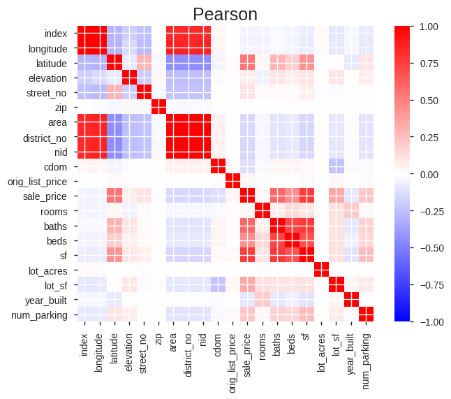
The features highly correlated with sale price include latitude, bathrooms, bedrooms, home square footage, lot square footage and parking. This makes sense as the northern portion of San Francisco has the priciest homes (latitude), homes with more square footage/beds/baths will fetch a higher price and parking is at a premium in San Francisco.
The Metrics
Since linear regression ended up being the selected model (more on model selection later), the key metrics are Mean Absolute Error (MAE) and R-Squared.
As a baseline, the MAE using the mean sale price for 2018 sales is $684,458. In other words, if I use the average price of a single-family home in San Francisco in 2018 as the prediction for every home the average error will be $684,458. The model better be able to beat this!
I also wanted to compare the model to Zillow’s results. They actually publish accuracy results for the San Francisco metro area (Zestimate metrics). While the results are not directly comparable to my data (the metro area is much larger), they do provide a rough stretch goal for the model.
- Median Error – 3.6%
- Zestimate Within 5% of Sale Price – 62.7%
- Zestimate Within 10% of Sale Price – 86.1%
- Zestimate Within 20% of Sale Price – 97.6%
The Evaluation Protocol
The evaluation protocol will divide the data set into a training set using data from 2009 – 2016, a validation set using 2017 data and a final test set using 2018 data.
- Train – 15,686 home sales from 2009 – 2016.
- Validate – 1,932 homes sales in 2017.
- Test – 1,897 home sales in 2018.
Model Selection
Linear regression models are well-documented as strong models for home price predictions and this was the initial model selected. A simple linear regression was performed with a minimum of data cleaning/wrangling and the results recorded. Both logistic regression and random forest models were also tried for comparison purposes and the linear regression model was clearly the leader. As the project progressed, I would periodically check it against a random forest model and the linear regression model continued to outperform the random forest model. So linear regression it is!
Developing the Model
The initial model was run using all the features with the results below. In order to see how well the model could perform I added a price per square foot feature which is actually a proxy sale price of the property. As expected, the results were great with price per square foot, but clearly unusable as the value will not be known when predicting prices in 2018. This is a clear example of data leakage.
| Initial Model | Overfit | |
|---|---|---|
| MAE | $400,376 | $219,266 |
| R-Squared | 0.6258 | 0.8971 |
The metrics from these initial predictions provide a base minimum and maximum to work with. In other words, I have a minimum that already beats the baseline and a maximum to shoot for using data wrangling to avoid the data leakage.
Data Wrangling
The key to optimizing the model lies in the data wrangling!
Eliminate Features
It turns out over 20 features had little or no impact on the predictions and could be removed thereby greatly simplifying the model. For example, city and state are the same for all properties.
Dates and Time Series
There are two date features in the data: sale date and on-market date. The on-market date is the day the property is listed on the MLS and has little impact on the predictions, so it was eliminated.
For sale date the year is needed as the data is split by year sold. This also brought up the issue of using a time series to forecast the prices. Unlike stocks with daily prices, real estate sales might happen once every 5-10 years. In order to use a time series, the model would need to use a price index that would take into account appreciation/depreciation and any seasonality. This approach was briefly tried, but the results were weak compared to my final model. The annual price multiplier is shown below. If you bought a home in San Francisco in 2009-2011 it has, on average, doubled in value by 2018!
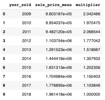
Ultimately only the year sold was used in the final model.
Zeros and Nans
Zeros and Nans in latitude, longitude, elevation, rooms, baths, lot square feet and lot acres were filled using a variety of methods (see code).
Feature Engineering
Eliminating features and filling zeros and Nans provided incremental improvements on the model, but feature engineering was required to obtain larger improvements.
Categorical data was encoded using OrdinalEncoding, but a few features improved the model by counting the number of categorical values in the features. For example, the views feature contained a list of all the potential views from a property picked from a list of 25 view types. It was reasoned that a property with more views would be more valuable. So, a view count feature was engineered to count the number of views recorded in the view feature. The same approach was used for parking and driveway/sidewalk features.
The key engineered feature, however, turned out to be the comparable sales feature. This feature is an estimated value created by simulating the way an agent would value a property. The code below takes the most recent sales of the nearest three properties of similar size (comparable sales) and calculates their average price per square foot which is used later in the model to calculate the comparable sale price. To avoid any data leakage, no 2018 comparable sales were used (the maximum comparable sale year is 2017).
nhoods = X[['sf', 'longitude', 'latitude']]

def neighbor_mean(sqft, source_latitude, source_longitude):

  source_latlong = source_latitude, source_longitude
  source_table = train[(train['sf'] >= (sqft * .85)) & (train['sf'] <= (sqft * 1.15))]
  target_table = pd.DataFrame(source_table, columns = ['sf', 'latitude', 'longitude', 'year_sold', 'sale_price'])

  def get_distance(row):
      target_latlong = row['latitude'], row['longitude']
      return get_geodesic_distance(target_latlong, source_latlong).meters

  target_table['distance'] = target_table.apply(get_distance, axis=1)

  # Get the nearest 3 locations
  nearest_target_table = target_table.sort_values(['year_sold', 'distance'], ascending=[False, True])[1:4]

  new_mean = nearest_target_table['sale_price'].mean() / nearest_target_table['sf'].mean()
  if math.isnan(new_mean):
    new_mean = test['sale_price'].mean() / test['sf'].mean()

  return new_mean

nhoods['mean_hood_ppsf'] = X.apply(lambda x: neighbor_mean(x['sf'], x['latitude'], x['longitude']), axis=1)
nhoods = nhoods.reset_index()
nhoods = nhoods.rename(columns={'index': 'old_index'})
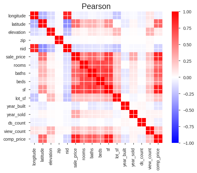
A new correlation matrix shows the resulting relationships of the new wrangled and engineered features.
Final Results
Finally, the model was run against the 2018 test data. The model had a test MAE of $276,308 and a R-Squared value of .7981 easily beating the baseline.
| Baseline | Validation | Test | |
|---|---|---|---|
| MAE | $400,376 | $249,452 | $276,308 |
| R-Squared | 0.6258 | 0.8364 | 0.7981 |
Compared against the Zestimate performance, the Jestimate model had a lower Median Error, but could not beat Zestimate’s strong distribution of errors. Again, the Zestimate data covers a larger territory than Jestimate.
| Jestimate | Zestimate | |
|---|---|---|
| Median Error | -1.7% | 3.6% |
| Within 5% | 21.3% | 62.7% |
| Within 10% | 43.5% | 86.1% |
| Within 20% | 75.5% | 99.5% |
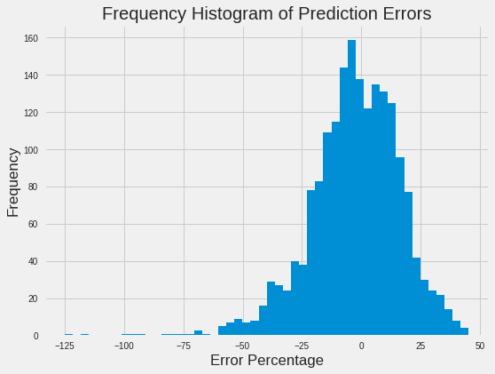
A histogram of the Jestimate percentage prediction errors shows the distribution:
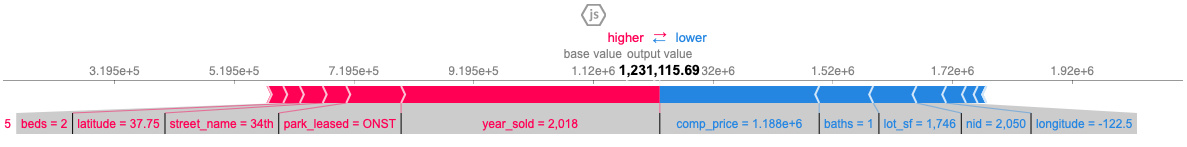
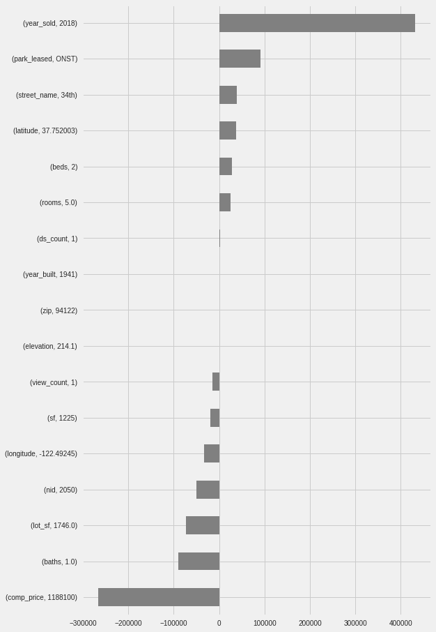
Feature Importance Using Shapley Values
In order to provide further insights into the predictions, the Shapley values were calculated for each property showing the features and their values having the highest positive impact (Pros) and the highest negative impact (Cons) on the predicted price.
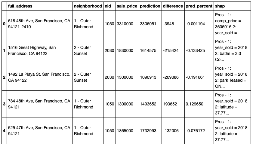
Display
A final display dataframe was created and saved in a .csv file for use by the display code. A separate article provides details on creating the interactive display of the data using Bokeh maps, data tables, and text fields.
This article was published on Towards Data Science on October 22, 2019 and can be viewed here.
This is Part of a Series of Articles Exploring San Francisco Real Estate Data
San Francisco Real Estate Data Source: San Francisco MLS, 2009-2018 Data