A decision tree is a popular and powerful method for making predictions in data science. Decision trees also form the foundation for other popular ensemble methods such as bagging, boosting and gradient boosting. Its popularity is due to the simplicity of the technique making it easy to understand. We are going to discuss building decision trees for several classification problems. First, let’s start with a simple classification example to explain how a decision tree works.
The Code
While this article focuses on describing the details of building and using a decision tree, the actual Python code for fitting a decision tree, predicting using a decision tree and printing a dot file for graphing a decision tree is available at my GitHub.
A Simple Example
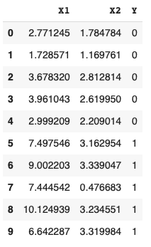
Let’s say we have 10 rectangles of various widths and heights. Five of the rectangles are purple and five are yellow. The data is shown below with X1 representing the width, X2 representing the height and Y representing the classes of 0 for purple rectangles and 1 for yellow rectangles:
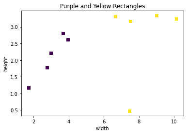
Graphing the rectangles we can very clearly see the separate classes.
Based on the rectangle data, we can build a simple decision tree to make forecasts. Decision trees are made up of decision nodes and leaf nodes. In the decision tree below we start with the top-most box which represents the root of the tree (a decision node). The first line of text in the root depicts the optimal initial decision of splitting the tree based on the width (X1) being less than 5.3. The second line represents the initial Gini score which we will go into more detail about later. The third line represents the number of samples at this initial level - in this case 10. The fourth line represents the number of items in each class for the node - 5 for purple rectangles and 5 for yellow rectangles.
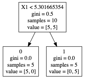
After splitting the data by width (X1) less than 5.3 we get two leaf nodes with 5 items in each node. All the purple rectangles (0) are in one leaf node and all the yellow rectangles (1) are in the other leaf node. Their corresponding Gini score, sample size and values are updated to reflect the split.
In this very simple example, we can predict whether a given rectangle is purple or yellow by simply checking if the width of the rectangle is less than 5.3.
The Gini Index
The key to building a decision tree is determining the optimal split at each decision node. Using the simple example above, how did we know to split the root at a width (X1) of 5.3? The answer lies with the Gini index or score. The Gini index is a cost function used to evaluate splits. It is defined as follows:
The sum of p(1-p) over all classes, with p the proportion of a class within a node. Since the sum of p is 1, the formula can be represented as 1 - sum(p squared). The Gini index calculates the amount of probability of a specific feature that is classified incorrectly when randomly selected and varies between 0 and .5.
Using our simple 2 class example, the Gini index for the root node is (1 - ((5/10)^2 + (5/10)^2)) = .5 - an equal distribution of rectangles in the 2 classes. So 50% of our dataset at this node is classified incorrectly. If the Gini score were 0, then 100% of our dataset at this node would be classified correctly (0% incorrect). Our goal then is to use the lowest Gini score to build the decision tree.
Determining the Best Split
In order to determine the best split, we need to iterate through all the features and consider the midpoints between adjacent training samples as a candidate split. We then need to evaluate the cost of the split (Gini) and find the optimal split (lowest Gini).
Let’s run through one example of calculating the Gini for one feature:
- Sorting X1 in ascending order we get the first value of 1.72857131
- For class 0, the split is 1 to the left and 4 to the right (one item <= 1.72857131, four items > 1.72857131)
- For class 1, the split is 0 to the left and 5 to the right (zero items <= 1.72857131, five items > 1.72857131)
- The left side Gini is (1 - ((1/1)^2 + (0/1)^2) = 0.0
- The right side Gini is (1 - ((4/9)^2 + (5/9)^2) = 0.49382716
- The Gini of the split is the weighted average of the left and right sides (1 * 0) + (9 * 0.49382716) = .44444444
Running this algorithm for each row gives us all the possible Gini scores for each feature:
| Feature | Value | Gini |
|---|---|---|
| X1 | 1.728 | .5000 |
| X1 | 2.771 | .4444 |
| X1 | 2.999 | .3750 |
| X1 | 3.678 | .2857 |
| X1 | 3.961 | .1666 |
| X1 | 6.642 | .0000 |
| X1 | 7.444 | .1666 |
| X1 | 7.497 | .2857 |
| X1 | 9.002 | .3750 |
| X1 | 10.12 | .4444 |
| X2 | 0.476 | .5000 |
| X2 | 1.169 | .4444 |
| X2 | 1.784 | .5000 |
| X2 | 2.209 | .4761 |
| X2 | 2.619 | .4166 |
| X2 | 2.812 | .4199 |
| X2 | 3.162 | .2666 |
| X2 | 3.234 | .2857 |
| X2 | 3.319 | .3750 |
| X2 | 3.339 | .4444 |
If we look at the Gini scores, the lowest is .0000 for X1 = 6.642 (class 1). We could use 6.642 as our threshold, but a better approach is to use the adjacent feature less than 6.642, in this case X1 = 3.961 (class 0), and calculate the midpoint as this represents the dividing line between the two classes. So, the midpoint threshold is (6.642 + 3.961) / 2 = 5.30! Our root node is now complete with X1 < 5.30, a Gini of .5, 10 samples and 5 in each class.
Building the Tree
Now that we have the root node and our split threshold we can build the rest of the tree. Building a tree can be divided into two parts:
- Terminal Nodes
- Recursive Splitting
Terminal Nodes
A terminal node, or leaf, is the last node on a branch of the decision tree and is used to make predictions. How do we know when to stop growing a decision tree? One method is to explicity state the depth of the tree - in our example set depth to 1. After our first split we stop building a tree and the two split nodes become leaves. Deeper trees can become very complex and overfit the data.
Another way a tree can stop growing is once the Gini is 0 - then no more splits are necessary. In our example, the depth is 1 and the Gini is 0 for the two leaves, so both methods of achieving termination are met. If we look at the terminal nodes we can see our predictors. If the width of the rectangle (X1) is less than 5.30, then moving to the left of the tree we see that the predicted class is 0 or a purple rectangle. If the width of the rectangle (X1) is greater than 5.30, then moving to the right of the tree we see the predicted class is 1 or a yellow rectangle.
Recursive Splitting
Now that we know when to stop building a decision tree, we can build the tree recursively. Once we have the root node, we can split the node recursively left and right until the maximum depth reached. We have all the basic building blocks from our simple example, but to demonstrate recursive splitting we will need a more complex example. Let’s use the famous, and somewhat tired, Iris data set as it is easily available in scikit for comparison purposes.
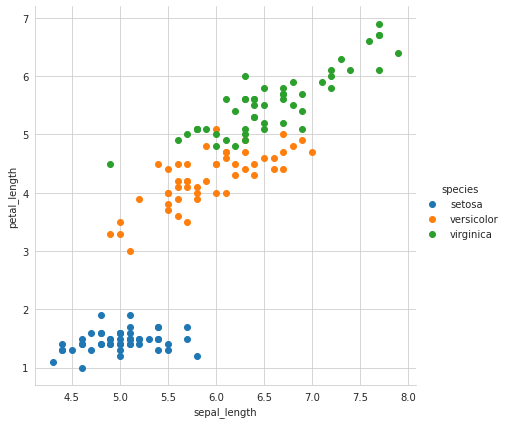
Graphing the Iris data we can clearly see the three classes (Setosa, Versicolor and Virginica) across two of the four features - sepal_length and petal_length:
Let’s create a Decision Tree recursively and see what the results look like.
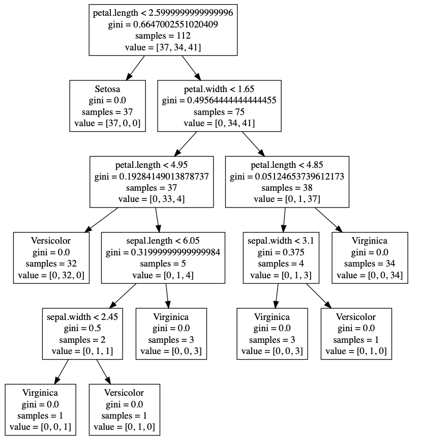
At the root node we have a first split of petal_length < 2.6 creating a leaf node with a Gini of 0.0 for Setosa and a decision node requiring a new split. We can clearly see the Setosa split in the graph at the midpoint between Setosa and Versicolor (petal_length = 2.6). Since the Gini is 0 for the left node, we are done and the leaf node is created just as we did with our rectangles. On the right side however, our right node has a Gini of .495. Since we have the depth set to 5, we recursively split again on the right node. This continues until we hit a depth of 5, producing the decision tree we see in the graph.
Pruning a Decision Tree
One downside of decision trees is overfitting. With enough depth (splits), you can always produce a perfect model of the training data, however, it’s predictive ability will likely suffer. There are two approaches to avoid overfitting a decision tree:
- Pre-pruning - Selecting a depth before perfect classification.
- Post-pruning - Grow the tree to perfect classification then prune the tree.
Two common approaches to post-pruning are:
- Using a training and validation set to evaluate the effect of post-pruning.
- Build a tree using a training set, then apply a statistical test (error estimation or chi-squared test) to estimate whether pruning or expanding a particular node improves the results.
Articles Referenced for code and data Include: