NFL fantasy football is a game in which football fans take on the role of the coach or general manager of a pro football team. Participants draft their initial teams, select players to play each week and trade players in order to compete weekly during a season against other teams. The winning teams are determined by the real-life statistics of the pro athletes.
Goal of the Trade Analyzer
The goal of the trade analyzer is to determine if a proposed trade of one or more players is a “good” or “bad” trade during any week of the 2019 football season. A good trade is defined as trading a player on your team for a player with higher expected fantasy football points. The goal, therefore, is to determine the expected fantasy football points of each pro football player for each week of the 2019 season. The expected points can then be compared between players. Use the Trade Analyzer app below or click here.
The Points System
The trade analyzer uses the ESPN Standard League rules for determining fantasy football points. A team consists of 9 starters in 7 position. The 7 postions are quarterback(QB), running back(RB), wide receiver(WR), tight end(TE), kicker(K) and team defense(DF). A team’s defensive squad is considered one “player” in fantasy football.
| QB/RB/WR/TE | Kickers | Defense and Special Teams |
|---|---|---|
| 6 pts rush or receive TD | 5 pts 50+ yard FG made | 6 pts def/special teams TD |
| 6 pts returning kick/punt for TD | 4 pts 40-49 yard FG made | 2 pts interception |
| 6 pts player ret/rec fumble for TD | 3 pts FG made 39 yards or less | 2 pts fumble recovery |
| 4 pts passing TD | 2 pts rush/pass/rec 2 pt. conv | 2 pts blocked punt/PAT/FG |
| 2 pts rush/receive 2 pt. conv | 1 pt extra point made | 2 pts safety |
| 2 pts passing 2 pt. conversion | -1 pt missed FG | 4 pts 1-6 points allowed |
| 1 pts 10 yards rush or receive | 3 pts 7-13 points allowed | |
| 1 pt 25 yards passing | 1 pts 14-17 points allowed | |
| 2 pts rush or receive TD of 40+ yds | 0 pts 18-27 points allowed | |
| 2 pts passing TD of 40+ yds | -1 pts 28-34 points allowed | |
| -2 pts interception | -3 pts 35-45 points allowed | |
| -2 pts fumble lost | -5 pts 46+ points allowed | |
| 1 pt per sack |
Data
The data used for modeling came from ArmchairAnalysis.com. The data consists of over 700+ data points over 28 different excel tables providing 20 years of detailed stats for every player in the NFL since the year 2000.
The raw data was initially manipulated in Excel in order to link and extract the relevant data for all 2019 NFL players. The manipulated data formed the basis for the initial modeling data. From the initial modeling data the actual fantasy football points were calculated for each game of each season for every 2019 player. The training data for the models used all the data available for each player up through the 2018 season with the 2019 data used as the test data. For example, if a player began his pro career in 2014, then 2014 - 2018 data was used for training data and 2019 data was used for test data.
Modeling
A total of four models were employed in predicting expected fantasy football points for 653 2019 NFL players. The data is essentially time-series data with players having anywhere from 0 to 20 years (20 seasons x 16 games = 320 data points) of data.
-
Average - A baseline measure was established using an average for each 2019 player. The week 1 average was established using the average points per game for the players during the 2018 season (excluding rookies). Weeks 2 through 17 were calculated using the average of their actual performance from previous weeks (e.g. week 2 used week 1 actual performance, week 3 used the average of week 1 and 2 actuals, etc.). This would be considered the naive approach and one often used by the average fantasy football participant.
-
XGBoost - An XGBoost model was used to predict rookie player performance in week 1 of the 2019 season. The 106 2019 rookies are difficult to predict as they have no professional experience. Using the rookie year stats for the 515 non-rookie players (excluding defense) as training data, week 1 expected fantasy points for the 2019 season were calculated with a validation MAE of 28.93 and R-squared of .49 and a test MAE of 30.75 and R-squared of .43. These were weak results, but a starting point was needed. Weeks 2 through 17 were calculated using the average of their actual performance from previous weeks - the same as the baseline (e.g. week 2 used week 1 actual performance, week 3 used the average of week 1 and 2 actuals, etc.).
-
ARIMA - An ARIMA model was initially used to predict veteran player performance for each week in the 2019 season. Only veteran players with over 3 years of experience and at least 50 points during the 3 years were run using ARIMA as the model needs about 50 data points (3 seasons x 16 games = 48 data points) to perform well. About 246 veteran players were modeled using ARIMA and while the results were very good (see the Evaluate tab) and beat the baseline, the neural network model showed better results.
-
Recurrent Neural Network, Long Short-Term Memory (RNN-LSTM) - A RNN-LSTM model was used to predict veteran player performance for each week in the 2019 season. Only veteran players with over 3 years of experience and at least 50 points during the 3 years were run using RNN-LSTM as the model needs as much data as possible and 3 years seemed to be a good balance. About 246 veteran players were modeled using RNN-LSTM and the results compared to the ARIMA model. The RNN-LSTM model outperformed both the baseline average and the ARIMA models and was the model used in the final app.
Notes:
-
Final Results - The final results combine the rookie results(XGBoost+Average - 106 players), the veterans with 3+ years(RNN-LSTM - 278 players including defense) and the remaining veterans with < 3 years experience(Average - 269 players). This is referred to as the “NN” model in the Evaluate tab and the “ARIMA” is the same combination of results only using ARIMA for the veterans with 3+ years.
-
Weekly Predictions - The models each calculate predictions for each of the remaining weeks of the season. Each remaining week is then summed to arrive at the players expected fantasy football points. For example, in week 1 the expected fantasy football points are the sum of all 16 game predictions (the entire season), in week 2 the points are the sum of the 15 remaining games, etc.
-
Bye Weeks - There are actually 17 weeks in a football season and each team has a random bye week during the season. On bye weeks, each player’s prediction from the week before is simply carried forward.
-
Injuries - Injuries play a huge role in fantasy football. When a player is injured his points essentially fall to zero. There is no reliable way to forecast if or when a player will get injured. While the raw data does provide some details on injuries, it still does not provide good information on when a player will return from an injury. In all the models, when a player goes on injured reserve status, he is assumed to be out for the season.
The Code
All the code, data and associated files for the project can be accessed at my GitHub repo. The README file provides details of the repo directory and files.
The RNN-LSTM Model
While the complete code for predicting fantasy football points is quite involved, let’s take a closer look at the core RNN-LSTM code using one player as an example. We are going to use Aaron Rodgers, the quarterback for the Green Bay Packers. Aaron is an excellent test case as he started his NFL career in 2005 providing 15 years of data. In addition, he did not suffer any significant injuries during the 2019 season.
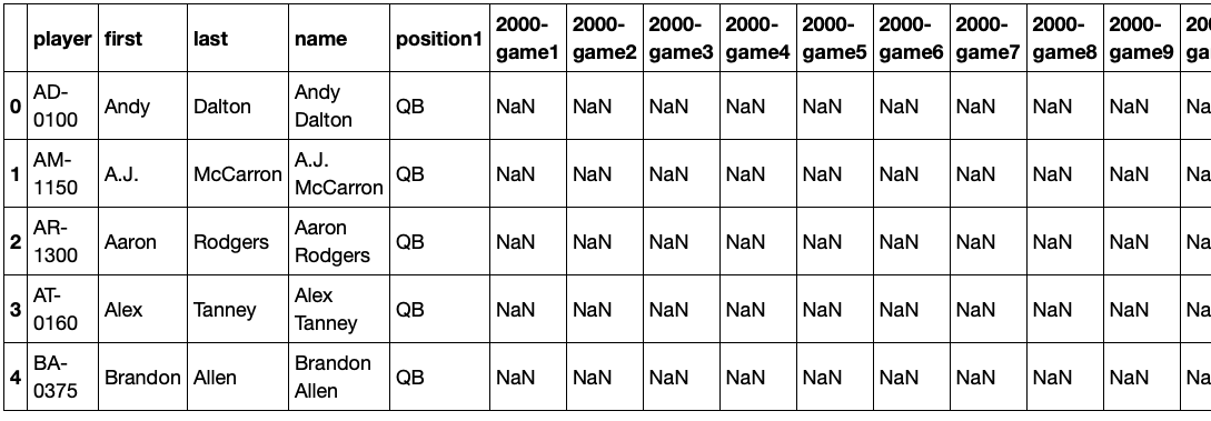
The actual points for each 2019 NFL player is stored in the original_df dataframe. The first five columns of the dataframe contain descriptive features for each player. The next 320 columns contain the actual fantasy football points for each game from 2000 to 2019 for each player (16 games per season x 20 seasons = 320 data points). These values are NaN until the player’s first NFL season. So Aaron Rodgers actual data does not begin until column 85 (16 x 5 = 80 games until the 2005 season plus the 5 descriptive columns).
The initial call to the RNN-LSTM prediction function lstm_pred occurs in the function named main. The input to the function consists of:
player = ‘Aaron Rodgers’ (This is the name of the player)
n_periods = 16 (In this example we are beginning at the start of the season and predicting all 16 games of the 2019 season)
col = 85 (Aaron’s 2005 data begins in the 85th column of the dataframe)
pred_points = lstm_pred(player, n_periods, col)
Using these three inputs, let’s take a close look at lstm_pred.
def lstm_pred(p, np, c):
    series = make_series(p, c)
    X = series.values
    supervised = timeseries_to_supervised(X, 1)
    supervised_values = supervised.values

    # Split data into train and test-sets
    train, test = supervised_values[0:-np], supervised_values[-np:]

    # Transform the scale of the data
    scaler, train_scaled, test_scaled = scale(train, test)

    # Fit the model
    lstm_model = fit_lstm(train_scaled, 1, 100, 1)

    # Forecast the entire training dataset to build up state for forecasting
    train_reshaped = train_scaled[:, 0].reshape(len(train_scaled), 1, 1)
    lstm_model.predict(train_reshaped, batch_size=1)

    # Walk-forward validation on the test data
    yhat_sum = 0
    for i in range(len(test_scaled)):
        # Make one-step forecast
        X, y = test_scaled[i, 0:-1], test_scaled[i, -1]
        yhat = forecast_lstm(lstm_model, 1, X)
        # Invert scaling
        yhat = invert_scale(scaler, X, yhat)
        # Sum the weekly forecasts
        yhat_sum = yhat_sum + yhat

    return yhat_sum
Let’s walk through this code to better understand how it works. The first four lines are simply preparing the data for the model.
series = make_series(p, c)
X = series.values
supervised = timeseries_to_supervised(X, 1)
supervised_values = supervised.values
The function make_series simply converts Aaron’s actual points stored in the dataframe from 2005 through 2019 into a python Series. The values of the series are then stored in X. The X values now represents our time series for Aaron’s fantasy football points. The function timeseries_to_supervised(X, 1) takes the time series X and creates a dataframe containing X our supervised learning input pattern and y our supervised learning output pattern. The y values are simply the X series shifted back one period. The X and y values are then stored in the numpy array supervised_values. What we’ve done with these four lines of code (and their functions) is taken Aaron’s fantasy football point production from the original_df dataframe and converted it into a form for supervised learning. The tail end of the supervised_values representing the 2019 season is below. The first column represents the X values and the second column the y values.
 ....
 [ 1.04 12.92]
 [12.92 14.36]
 [14.36 14.3 ]
 [14.3  25.48]
 [25.48  9.42]
 [ 9.42 18.32]
 [18.32 44.76]
 [44.76 28.1 ]
 [28.1  12.94]
 [12.94 10.02]
 [10.02  9.46]
 [ 9.46 28.12]
 [28.12 11.4 ]
 [11.4  14.42]
 [14.42  9.34]
 [ 9.34 19.02]]
The next line of code splits the supervised_values into train and test splitting off the last 16 games (the 2019 season) into the test set and leaving the 2005 - 2018 seasons as the training set.
train, test = supervised_values[0:-np], supervised_values[-np:]
Once the code is split, the data is normalized using the scale function. The scale function uses the MinMaxScaler with a range of (-1,1). Normalizing the data is recommended as it should make learning easier for a neural network and should ensure the magnitude of the values are more or less similar.
scaler, train_scaled, test_scaled = scale(train, test)
We are now ready to fit the RNN-LSTM model passing the function fit_lstm the following parameters:
train - train_scaled
batch_size - 1
nb_epochs - 100
neurons - 1
lstm_model = fit_lstm(train_scaled, 1, 100, 1)
The fit_lstm function is where the RNN-LSTM magic happens. In a nutshell, the function uses a Sequential Keras API with a LSTM layer and a Dense layer. The loss function used is “mean squared error” with the “adam” optimization algorithm. The actual mechanics of the function are quite involved and for those wishing to obtain further information please see the detailed description of the function found in the LSTM Model Development section of the article Time Series Forecasting with the Long Short-Term Memory Network in Python by Jason Brownlee whose code I borrowed for this function.
The article recommends a higher number of epochs (1000 - 4000) and neurons (1-5) for better results, but due to time and resource requirements of running forecasts for several hundred players, the 100 epochs and 1 neuron provided very good results in a less resource intensive manner.
We are now ready to make forecasts using the lstm_model.predict function of the model.
train_reshaped = train_scaled[:, 0].reshape(len(train_scaled), 1, 1)
lstm_model.predict(train_reshaped, batch_size=1)
The function requires a 3D numpy array as input and in our case this will be an array of one value (the observation of the previous time step) and outputs a 2D numpy array of one value. Before we forecast the test data we need to seed the initial state by making a prediction of all the values in the training data. The first line of the code above reshapes the data into the one value 3D numpy array and the second line sets the initial state for the network using the training data.
All we have left is to step through the test data, make individual forecasts for the 16 games, and invert the scaling to arrive at the final individual predictions. The individual predictions are then summed to create the predicted fantasy football points for Aaron’s 2019 season.
yhat_sum = 0
for i in range(len(test_scaled)):
    # Make one-step forecast
    X, y = test_scaled[i, 0:-1], test_scaled[i, -1]
    yhat = forecast_lstm(lstm_model, 1, X)
    # Invert scaling
    yhat = invert_scale(scaler, X, yhat)
    # Sum the weekly forecasts
    yhat_sum = yhat_sum + yhat
The predicted results for Aaron Rodgers season are below. The total prediction for the season is 293 (rounded) and his actual points were 282 - a not bad 4% error for the season! (Results will vary slightly each time the code is run)
yhat =  13.550041856765747
yhat =  15.615552995204924
yhat =  17.195858060121534
yhat =  18.015674024820328
yhat =  20.544238206744193
yhat =  18.375679302811623
yhat =  19.83470756918192
yhat =  18.937192922234534
yhat =  21.3260236287117
yhat =  20.56778145074844
yhat =  18.166402292251586
yhat =  16.316439254283903
yhat =  19.98121999800205
yhat =  18.90507374048233
yhat =  18.95989200234413
yhat =  16.812043523192404

yhat_sum =  293.10382082790136
An Evaluation of the Model Predictions
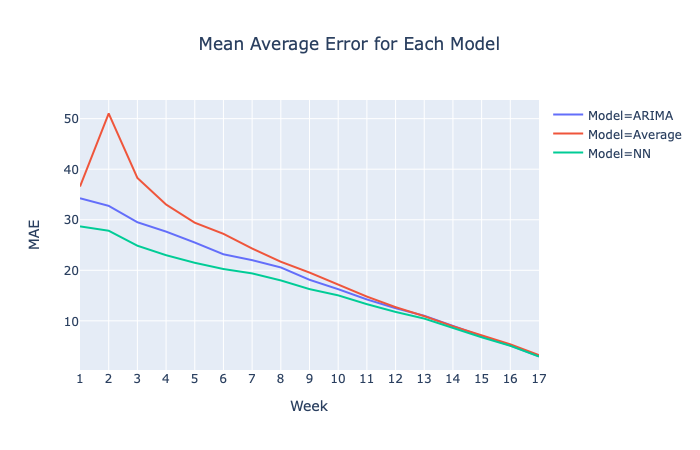
The Recurrent Neural Network - LSTM Model(NN) outperforms both the baseline Average and ARIMA models. While both the NN and ARIMA models have lower MAEs they all start to converge about halfway through the season as all models incorporate the current season actual points and the number of future predictions are reduced thereby increasing accuracy in all the models.
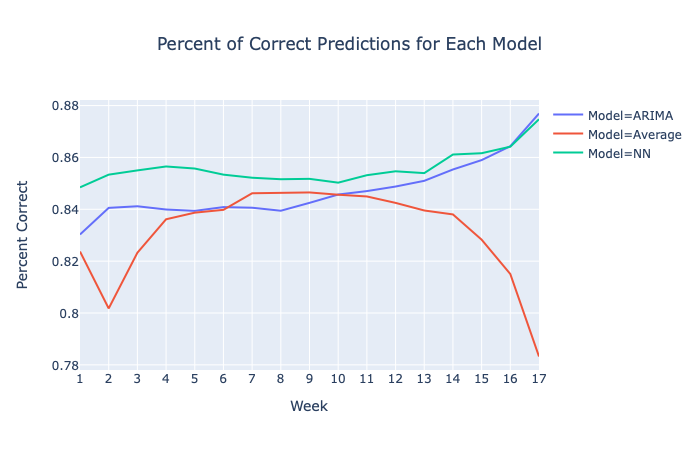
The real accuracy of the models are shown in the Percent of Correct Predictions graph. For each week, the predicted outcome of a “good” or “bad” trade for each player is calculated against every other player and compared with the actual outcome. The NN clearly makes better predictions over the other models with an overall average correct percentage of 85.59% for the 2019 season compared with 84.72% for an ARIMA model and 83.17% for the baseline average model.
Fantasy Football Raw Data Souce: ArmchairAnalysis.com
RNN-LSTM Model Development: Time Series Forecasting with the Long Short-Term Memory Network in Python by Jason Brownlee
Image Credit: Pixabay