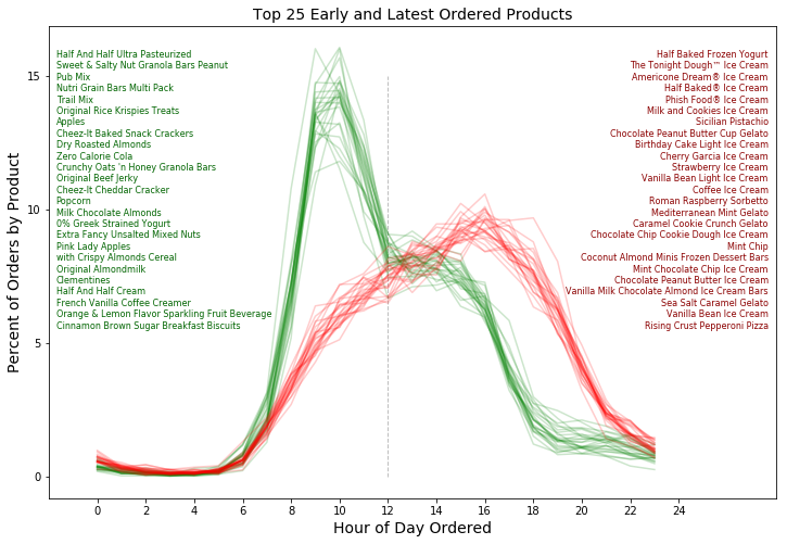
What are the most popular Instacart grocery products ordered early in the day? What are the most popular Instacart grocery products ordered late in the day? Early in the day, customers bought healthy items such as granola bars, while later in the day customers bought less healthy items such as ice cream!
Instacart released a public dataset, “The Instacart Online Grocery Shopping Dataset 2017”, containing anonymized data with a sample of over 3 million grocery orders from more than 200,000 Instacart users.
The data set can be accessed as follows: “The Instacart Online Grocery Shopping Dataset 2017”, Accessed from https://www.instacart.com/datasets/grocery-shopping-2017 on 7/26/2019. Questions: open_data@instacart.com.
One challenge was to graph the most popular products by hour of day ordered to find the top user purchases early in the day and late in the day.
Here is the completed chart:
Steps to Create the Graph
Here is the high level view for creating the graph.
Step 1 - Load the Data
The data can be downloaded as a .zip file containing 12 .csv files using the following commands in Colab notebook. The files are downloaded to the local notebook directory.
!wget https://s3.amazonaws.com/instacart-datasets/instacart_online_grocery_shopping_2017_05_01.tar.gz
!tar --gunzip --extract --verbose --file=instacart_online_grocery_shopping_2017_05_01.tar.gz
%cd instacart_2017_05_01
!ls -lh *.csv

-rw-r--r-- 1 502 staff 2.6K May  2  2017 aisles.csv
-rw-r--r-- 1 502 staff  270 May  2  2017 departments.csv
-rw-r--r-- 1 502 staff 551M May  2  2017 order_products__prior.csv
-rw-r--r-- 1 502 staff  24M May  2  2017 order_products__train.csv
-rw-r--r-- 1 502 staff 104M May  2  2017 orders.csv
-rw-r--r-- 1 502 staff 2.1M May  2  2017 products.csv
Step 2 - Merge the Data
Begin by merging the order_products_prior with order_products_train to create on order_products dataframe, then merge it with product and orders to gain the full base data.
Step 3 - Create a Top Products Dataframe
Create a new dataframe top_products with all products with orders greater than 2,900 and merge it with product to get a full subset of top products.
Step 4 - Create a Dataframe with Products Grouped by Hour of Day and Add Count and Percent Columns
Create a product_orders_by_hour dataframe grouped by product_id and order_hour_of_day. Add a sum column to count the number of orders each hour for each product and a percentage column to represent the percent of orders the sum equaled.
Step 5 - Create a Dataframe with the Mean Hour for Each Product
For each product in product_orders_by_hour, group by the average hour sum(order hour x # orders for hour)/total orders. This creates the mean_hour dataframe containing the product_id and mean_hour for all the products.
Step 6 - Sort the Mean Hour for Each Product to Create the Early and Late Lists
By sorting the mean_hour dataframe in ascending order and taking the top 25, you get the early_list dataframe containing the top 25 early products and by sorting in descending order and taking the top 25, you get the late_list dataframe containing the top 25 late products. Pull out the product names to create the early_product_names list and the late_product_names lists for the legends. Merge the early and late dataframes with product_orders_by_hour to get the early_pct and late_pct dataframes for plotting.
Step 7 - Plot the Results
Use early_pct and late_pct dataframes to plot the Order Hour of the Day against the Percent of Orders by Product. Use the early_product_names and late_product_names for the two legends.